
The free and powerful tool statisticians love
Data is now the lifeblood of any successful business. In this short article I’ll try to show how you can do powerful data analysis quickly and with relatively low effort using the open-source R programming language. Spreadsheets are nice, but R will take your data analysis skills to a whole different level. Don’t let the “Programming language” part deter you, you don’t need a computer science degree to use R. In fact R is the tool of choice for statisticians and quantitative analysts. On the flip side there’s a fair bit of depth to R and the ramp up curve can be steep. Hopefully this article will give you a taste and a starting point in your exploration.
What’s R?
R is an open-source programming language and software environment targeted at statistical computing, which means it’s brutally efficient at crunching large amounts of data and generating statistics and charts. It’s very popular with statisticians, quants, investors and anyone else that needs to explore, compute, chart, clean or manipulate data. Because it’s so popular there’s a thriving community of developers and practitioners around it, so for almost any problem you’re trying to solve there’s already a solution posted somewhere in developer forums or implemented in open source libraries called packages. There are packages for pretty much anything now, from statistics to machine learning to life sciences. There’s also a plethora of online resources from which to learn R. I will link to some at the bottom of this article.
You can download R here: https://cran.r-project.org/
It’s possible to program R directly from the command line, but most people use RStudio, a handy integrated development environment, which is also free and open-source.
A simple example — designing a movie blockbuster by the numbers
I’ve put together a simple “hello world” program to demonstrate a very tiny part of the capabilities of R. In this fictional example assume that you’re a film producer planning your next blockbuster project. Obviously you’re interested in maximizing profits, but today you decide to take a novel approach — use data to find what are makes movies successful.
This example will use movie dataset originating from IMDB.com which I downloaded from Kaggle.com (IMDB has an API for developers). It contains around 5000 movies with their metadata.
Note: We don’t know that the data is up-to-date or even very accurate, therefore the findings below should be assumed to be somewhat fictional too.
Importing and exploring data
You can import data into R from .csv files, or from other types of databases. I’ll use the function read.csv() to read the csv file I downloaded:
> movies <- read.csv(“movie_metadata.csv”, stringsAsFactors = TRUE)
This imported the data into a data frame called “movies”. Think of a data frame as of a single sheet in a spreadsheet. It has columns, which may be of different data types, and lines, each representing a movie in this case.
Note: for brevity I’m not going over all the details in each code snippet. For example the stringAsFactors = TRUE parameter is less relevant for our needs so I’ll leave it to you to read about it later if you wish.
Let’s see how many lines and columns we have.
> dim(movies)
[1] 4966 28
The dim (dimensions) function tells us there are 28 columns and 4966 lines, presumably one per movie in the dataset. Let’s take a closer look at the names of the columns.
> colnames(movies)
 [1] “color” “director_name” “num_critic_for_reviews”
 [4] “duration” “director_facebook_likes” “actor_3_facebook_likes”
 [7] “actor_2_name” “actor_1_facebook_likes” “gross”
[10] “genres” “actor_1_name” “movie_title”
[13] “num_voted_users” “cast_total_facebook_likes” “actor_3_name”
[16] “facenumber_in_poster” “plot_keywords” “movie_imdb_link”
[19] “num_user_for_reviews” “language” “country”
[22] “content_rating” “budget” “title_year”
[25] “actor_2_facebook_likes” “imdb_score” “aspect_ratio”
[28] “movie_facebook_likes”
So per movie we’re getting a lot of useful metadata — title, year, country duration, director, three leading actors, genre language etc. There’s some data specific to IMDB — number of critics, number of reviews and resulting IMDB score. Interestingly there are the number of Facebook Likes given to the movie, the director and the actors. Lastly, and perhaps most relevant to us, we budget and gross revenue per movie.
Now the fun begins. Let’s hypothesize that that IMDB scores play a big role in the success of a movie (we’ll check that later). But first what’s the normal range of IMDB scores that we should expect?
> summary(movies$imdb_score)
 Min. 1st Qu. Median Mean 3rd Qu. Max.
 1.600 5.800 6.600 6.425 7.200 9.300
The function summary gives some basic statistics: min value, 25%-ile, Median, Mean, 75%-ile and max value. Apparently in our sample no movie ever got a score greater than 9.3 or lower than 1.6. Looking at the numbers above we can imagine IMDB scores follow some normal bell-curve distribution with a middle point of 6.45. Let’s see:
> hist(movies$imdb_score, 100)
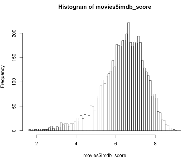
Yep, exactly, although the curve is not symmetric. Lastly let’s see what the minimal score wil put our movie in the top 10%. I’m using the function quantile() for this.
> quantile(movies$imdb_score, probs = 0.90, na.rm = TRUE)
90%
7.7
So now we have a better understanding of how IMDB scores are distributed and what we can expect.
Filtering and cleaning up data
Using irrelevant, missing or unclean data can greatly skew your analysis. With R filtering and cleaning that data is very straightforward.
Let’s say that the for the purpose of this analysis we’re only interested in movies produced in the USA. Are there other production countries in our dataset?
> levels(movies$country)
 [1] “” “Afghanistan” “Argentina” “Aruba”
 [5] “Australia” “Bahamas” “Belgium” “Brazil”
 [9] “Bulgaria” “Cambodia” “Cameroon” “Canada”
[13] “Chile” “China” “Colombia” “Czech Republic”
[17] “Denmark” “Dominican Republic” “Egypt” “Finland”
[21] “France” “Georgia” “Germany” “Greece”
[25] “Hong Kong” “Hungary” “Iceland” “India”
[29] “Indonesia” “Iran” “Ireland” “Israel”
[33] “Italy” “Japan” “Kenya” “Kyrgyzstan”
[37] “Libya” “Mexico” “Netherlands” “New Line”
[41] “New Zealand” “Nigeria” “Norway” “Official site”
[45] “Pakistan” “Panama” “Peru” “Philippines”
[49] “Poland” “Romania” “Russia” “Slovakia”
[53] “Slovenia” “South Africa” “South Korea” “Soviet Union”
[57] “Spain” “Sweden” “Switzerland” “Taiwan”
[61] “Thailand” “Turkey” “UK” “United Arab Emirates”
[65] “USA” “West Germany”
So 65 different production countries. Since we want only US films, lets copy those into a new data frame called “m”.
m <- movies[movies$country == “USA”, ]
That’s it. One line and an entire new data frame was created (you can create as many as you like of course). Let’s look at its dimensions.
> dim(m)
[1] 3747 28
So 3747 films were produced in the USA. Note that this data frame has the same 28 columns that the original “movies” had.
Next lets look at money — specifically the columns “budget” and “gross”
summary(m$budget)
Min.   1st Qu.    Median      Mean   3rd Qu.      Max.      NA's
218   6500000  20000000  35870000  50000000 300000000       251
> summary(m$gross)
Min.   1st Qu.    Median      Mean   3rd Qu.      Max.      NA's
703  10110000  32180000  55210000  72150000 760500000       512
We can see that budgets range from $218 to $300M and gross revenue from $162 to $760M. However we also see hundreds of “NA’s” (Not available), which indicate missing values. Let’s filter out films that are missing budget or gross.
> m <- m[is.na(m$gross) == FALSE, ]
> m <- m[is.na(m$budget) == FALSE , ]
> dim(m)
[1] 3074 28
We’re left with 3074 rows.
Calculating data
Let’s say that (rather naively) we’re measuring profit as the difference between gross revenue and budget. This is data we don’t yet have, but it’s very easy to get:
> profit <- m$gross — m$budget
This one command subtracted all 3074 values in the column “budget” from the corresponding 3074 values in the column “gross”. The result is a vector, an ordered array of elements, which I named “profit”. Let’s check the size of this vector:
> length(profit)
[1] 3074
As expected, there are 3074 elements in the profit vector.
Next lets see the distribution of movie profits.
> hist(profit, 100)
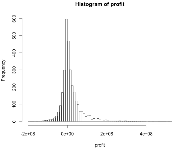
It looks as if most movies are just breaking even, and then there’s a normal distribution of winners and losers. Curious to see the movies that made 8 figures profit? To do this we‘ll first add the profit vector as a new column in “m”, our USA movies dataset, using the function cbind (column bind).
> m <- cbind(m, profit)
So we should now have a 29 columns, one of which called “profit”:
> dim(m)
[1] 3074 29
> colnames(m)
 [1] “color” “director_name” “num_critic_for_reviews”
 [4] “duration” “director_facebook_likes” “actor_3_facebook_likes”
 [7] “actor_2_name” “actor_1_facebook_likes” “gross”
[10] “genres” “actor_1_name” “movie_title”
[13] “num_voted_users” “cast_total_facebook_likes” “actor_3_name”
[16] “facenumber_in_poster” “plot_keywords” “movie_imdb_link”
[19] “num_user_for_reviews” “language” “country”
[22] “content_rating” “budget” “title_year”
[25] “actor_2_facebook_likes” “imdb_score” “aspect_ratio”
[28] “movie_facebook_likes” “profit”
Cool. Now we can check which titles racked in the money:
> m$movie_title[m$profit > 400000000]
[1] Star Wars: Episode IV - A New Hope
[2] The Avengers
[3] Avatar
[4] E.T. the Extra-Terrestrial
[5] Titanic
[6] Jurassic World
Interesting. Five big-budget sci-fi films and one big-budget romantic disaster movie. From this small sample we can naively guess that high budget leads to high profits. But does it?
Correlation? Causation?
Correlating data is an important part in any business analysis. R makes it very easy to do:
> cor(m$budget, m$profit, use=”complete.obs”)
[1] 0.0577743
The command cor() measures the correlation between two vectors. 1.0 is 100% full correlation. -1.0 is full inverse correlation. 0.0 is no correlation at all. A value of 0.0577743 basically means profits are not correlated with budget. You can’t predict if a movie will be a blockbuster just from its budget: high budget films can flop and low budget films can succeed. Let’s show this graphically by plotting the two values on the X and Y axis:
> plot(m$budget, m$profit)
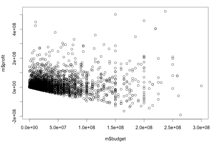
As you can see the dots are scattered all over with no clear pattern. There’s a concentration around zero because there are more samples there.
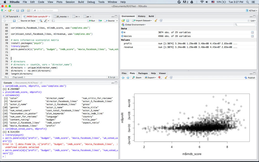
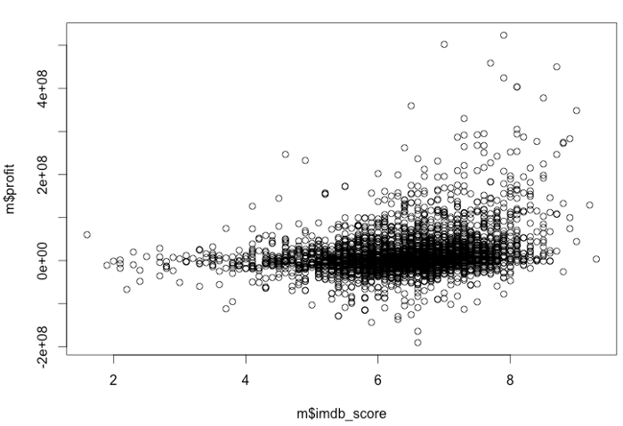
OK, let’s go back to our earlier theory then — is IMDB score a good predictor of profit?
> cor(m$imdb_score, m$profit, use=”complete.obs”)
[1] 0.2949907
Far from perfect, but the correlation is much stronger : 0.294. Graphically it looks like this:
Leveraging R Packages
What about Facebook Likes, are they a good predictor? What about the number of people that submitted votes in IMDB? We can do a bunch more 1:1 correlations, but actually there’s a better way to do it all and we don’t even have to code it. We’ll install a statistical package called “psych” that has just what we need.
install.packages(“psych”)
library(psych)
The function we’re after is called “pairs.panels()” — you just need to tell it which vectors to compare and it will generate an all-in-one result chart.
> pairs.panels(m[c(“profit”, “budget”, “imdb_score”, “movie_facebook_likes”, “num_voted_users”)])
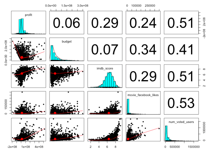
The columns and lines indicate the vectors being correlated. From left to right and from top to bottom: profit, budget, imdb_score, movie_facebook_likes, num_voted_users. The charts along the main diagonal show distribution histograms of each value. The numbers in the upper right boxes show the correlation value of the intersecting row and column. For example 0.34 is the correlation between movie budget and Facebook Likes. Similarly the boxes on the bottom left show scatter plots of the intersecting vectors.
Since we’re most interested in profits let’s look at the top line. As we saw before budget has almost no correlation with profit — 0.06. IMDB score and Facebook likes have a weak correlations (0.29 and o.24 respectively) with profits, and interestingly, the number of votes the movie got in IMDB is most strongly correlated with profits. Perhaps not surprising — a really successful movie is seen by more people which in turn yields more IMDB votes.
Beyond basic analysis
We can easily think of hundreds of other theories to test. Some may involve a combination of factors, for example is a well liked director plus a well liked lead actor a formula for success? Should we release a romantic comedy with specific keywords in the title? You can of course test all of these with R, but even better, you can let R find the patterns (if they exist) for you using machine learning. R has many package to train and develop prediction models and as long as you’re not trying to work on massive datasets you can very well use them from your personal computer.
The beginning of a journey?
There’s a LOT more to R of course. If you want to go deeper there’s no shortage of resources online. Here are a few good starting points:
R-tutorials: https://www.r-bloggers.com/how-to-learn-r-2/
Video tutorials
Quora discussion
Itamar Gilad (itamargilad.com) is a product consultant and speaker helping companies build high-value products. Over the past 15 years he held senior product management roles at Google, Microsoft and a number of startups.
If you prefer to receive posts like these by email sign up to my newsletter.